Our R&D department is dedicated to inventing novel technologies for e-commerce. Currently, we are focused on leveraging machine learning to categorize product images, making product searches on web stores more effortless. However, in our work and the e-commerce domain, we frequently encounter challenges concerning the availability of data. In this context, I will explore the implementation of data augmentation techniques to address this problem.
The problem with overfitting
Let’s start with why small datasets are a problem. You have probably come across this problem if you’ve ever tried to learn a machine learning model with little data, especially with deep learning models. Your model initially seems to learn well, predicting with >99% accuracy on the original dataset, but later when you evaluate your model on a new dataset, the accuracy drops to 50%. What is the problem?
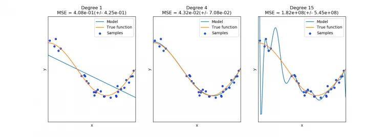
Let’s assume that we want to approximate some function — in this example — part of cosine function. These plots below show the function we want to approximate and represent two issues we might encounter. The left model uses a 1st-degree polynomial (a linear function), and we can clearly see that straight line is far from good approximation of cosine wave. This is known as underfitting. On the center plot, a 4th-degree polynomial is used to model the function with much better result and a small error. Finally, the far-right model is our object of interest. Using a 15th-degree polynomial, the model has the largest number of parameters, and because of this has a tendency to learn noise and/or remember specific features of individual samples. In other words, the model does not generalize well.
Deep learning models have huge number of parameters, for example AlexNet has 60 million parameters[1], while more recent architectures like Google Inception have fewer (about 5 million), they are still huge numbers[2]. To demonstrate how big a problem this is, we will try to train from noise.
Using a simple Python script I generate 400 consisting of only 28 x 28 images filled with noise.
import numpy as np
from PIL import Image

for i in range(100):
    noise = np.random.rand(28, 28, 3) * 255
    noise_img = Image.fromarray(noise.astype('uint8'))
    noise_img.save(str(i) + '.jpg')
Example output:

Then I split these images into 4 directories: a, b, c and d. For training, I used an image retraining example from the TensorFlow repository:
This script shows how to adapt a pretrained network to a new classification problem. It takes the InceptionV3 (or Mobilenet) model trained on ImageNet, and replaces the top fully connected layer with a “clean” new and train only this last layer. This technique is called transfer learning. In the case of classifying my 4 classes, it means that I have “only” 8196 parameters to learn. So let’s start training:
$ python retrain.py \
--bottleneck_dir=output/bottlenecks \
--how_many_training_steps 15000 \
--model_dir=inception \
--output_graph=output/retrained_graph.pb \
--output_labels=output/retrained_labels.txt \
--image_dir noise_dataset/
So I am learning for 15 000 steps from images in noise_dataset/ where I put my 4 directories (a, b, c, d) with noise images. You can find an explanation for parameters by typing in your CLI:
$ python retrain.py -hUsing Tensorboard you can visualize summaries with the command:
$ tensorboard --logdir /tmp/retrain_logs/tmp/retrain_logs is default path to log summaries.
Tensorboard view:
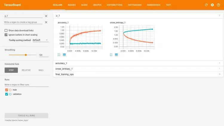

As you can see, our model has nearly 100% accuracy on training data, but on the validation set it’s even worse than a random model. 8196 parameters gives this model the capacity to remember all specific samples, which clearly shows why overfitting is big problem in deep neural networks.
This means that you need enormous datasets to train models like this, and most often these and similar models for training use the ImageNet dataset, which contains 1.2 million images. Nevertheless, overfitting can still occur, and there are some methods to deal with this problem, for example dropout[3], L1 and L2 regularization[4] and data augmentation[5].
Data augmentation
Data augmentation is a method by which you can virtually increase the number of samples in your dataset using data you already have. For image augmentation, it can be achieved by performing geometric transformations, changes to color, brightness, contrast or by adding some noise. Currently, there are ongoing studies on interesting new methods in data augmentation using Generative Adversarial Networks[6] or by pairing samples[7].
Why does data augmentation work? When and how should you use this technique to transform your data?
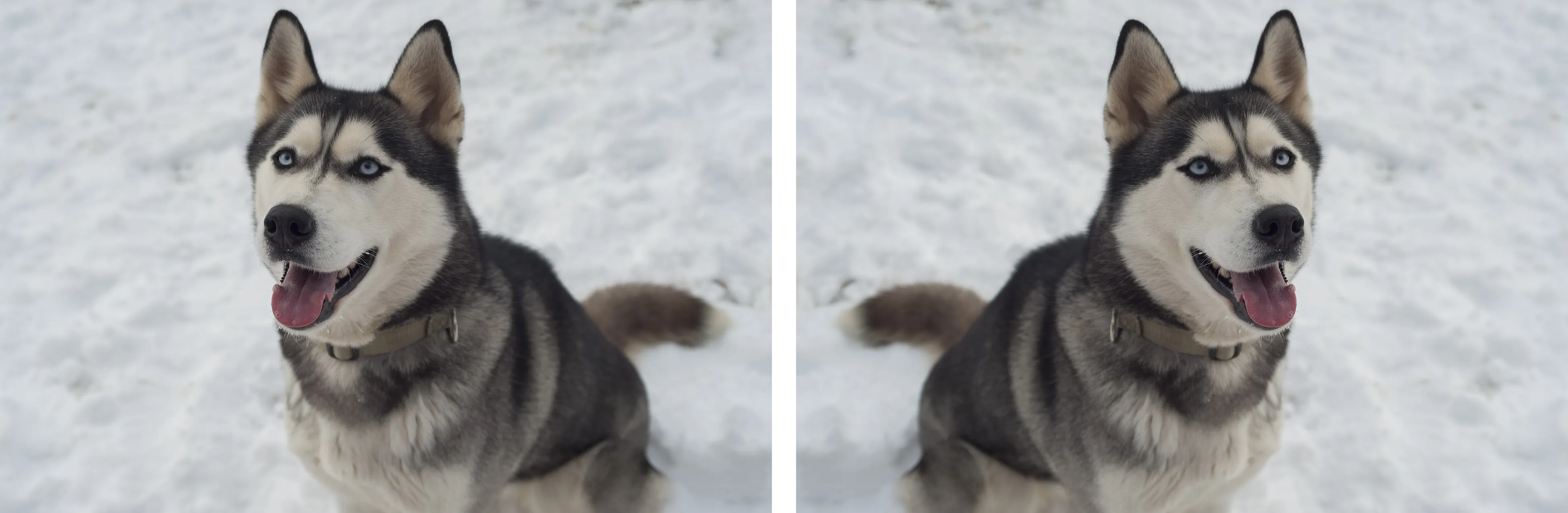
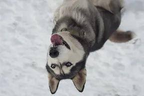
It is common knowledge in the field of machine learning algorithms that the more data you have, the better, even if the additional data is of worse quality. Data augmentation works because it adds prior knowledge, for example, in the two images below:
Flipping this photo doesn’t change its label — it is still a husky, but we have obtained a new sample in our data. Well, it may not be completely new, but we will come back to this later.
You should probably at least give data augmentation a try whenever you train a model. Even if your model has no symptoms of overfitting, data augmentation can also increase prediction accuracy. However, there are situations when data augmentation may change should be used with caution, such as in medical applications, because here, augmentation will change their labels. Since I don’t have much experience in the field of medical diagnosis, I have used more obvious example:
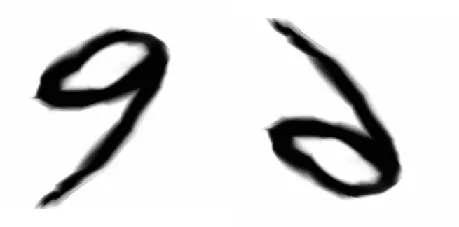
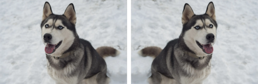
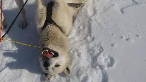
Here, flipping the left image has changed the meaning completely, from “nine” to a “six”. There are also some less obvious examples. Is there any sense of flipping our dog vertically? Its label won’t change but do you expect that photos like this will be fed into your application?
Probably not… but does it mean that this transformation doesn’t make sense? Well, it could increase inference accuracy with photos like this:
It’s important to note that data augmentation does not change the meaning of the samples, and it is crucial to keep in mind what kind of data inputs you expect for your app. For example, let’s assume that you have a dataset consisting mainly of good quality images, but you expect users to take worse quality photos with their phones, so you experiment by adding some noise, changing contrast and brightness to images in your dataset. But after training, you see that the validation accuracy has dropped. You may think that the model is not working, but this does not have to be true, because the photos in your validation are exclusively good quality images.
The experiment
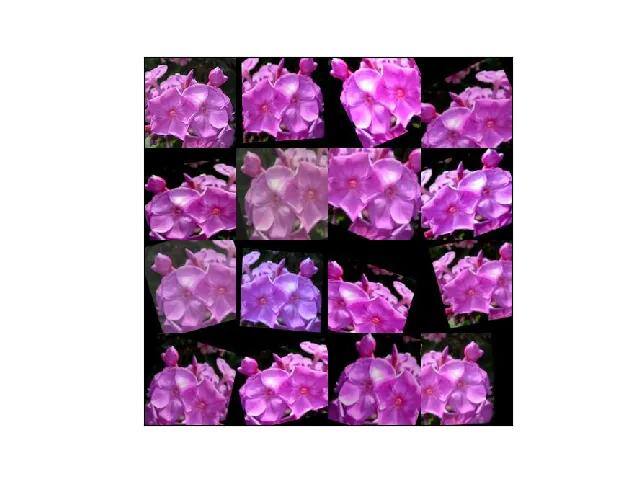
I have been looking for the right dataset for this article for a quite long time, because I wanted to show similar problems to the ones we encounter in our work at SNOW.DOG. While not completely ideal, I finally found one — the Flower Species Dataset. It’s a database made from fragments of photos of flowers, and reflects the flowering plants of different plant species.
You can download this dataset from Kaggle.
This dataset is really small, with only ~20 samples per class, but because the pretrained InceptionV3 model is very good at recognition species, it should be enough for transfer learning.
We will be using the same script for training that we use earlier to learn from noise, so we first have to prepare out dataset:
- change format of images to JPEG,
- split them to separate directories.
For converting I use Pillow.
import os
import csv

from PIL import Image

output = 'flower_split'

with open('flower_labels.csv') as csvfile:
    label_reader = csv.reader(csvfile, delimiter=',')
    next(label_reader)  # skipping header
    for row in label_reader:
        path = os.path.join(output, row[1])
        if not os.path.exists(path):
            os.makedirs(path)
        img = Image.open(row[0]).convert("RGB")
        dst = os.path.join(output, row[1], row[0].replace('.png', '.jpg'))
        img.save(dst)
As I have mentioned above, this dataset is not ideal, so to emphasize the problems we face in our own work, I changed optimizer from Gradient Descent to Adam in line 841 in retrain.py (you can read more about available TensorFlow optimizers here):
optimizer = tf.train.AdamOptimizer(FLAGS.learning_rate)
$ python retrain.py \
--bottleneck_dir=output/bottlenecks \
--how_many_training_steps 15000 \
--model_dir=inception \
--output_graph=output/retrained_graph.pb \
--output_labels=output/retrained_labels.txt \
--image_dir flower_split/ \
--learning_rate 0.0001
Learning for 15000 steps is probably too much but I want to have big margin for later reference, however learning shouldn’t take much time, even on CPU.

In Tensorboard there is option to smooth results which is useful especially in cases like this where there is little data. I wanted to visualise plots a little clearer using matplotlib, so I exported the data from Tensorboard and used the Savitzky–Golay filter for smoothing.
import numpy as np
import pandas as pd
import matplotlib.pyplot as plt
from scipy.signal import savgol_filter
train=pd.read_csv('run_train,tag_accuracy_1.csv', sep=',', header=0)
val=pd.read_csv('run_validation,tag_accuracy_1.csv', sep=',', header=0)
def annot_max(x, y, ax=None):
xmax = x[np.argmax(y)]
ymax = y.max()
text= "max={:.3f}".format(ymax)
if not ax:
ax=plt.gca()
bbox_props = dict(boxstyle="square,pad=0.3", fc="w", ec="k", lw=0.72)
arrowprops=dict(arrowstyle="->",connectionstyle="angle,angleA=0,angleB=60")
kw = dict(xycoords='data',textcoords="axes fraction",
arrowprops=arrowprops, bbox=bbox_props, ha="left", va="bottom")
ax.annotate(text, xy=(xmax, ymax), xytext=(0.75,0.75), **kw)
train_x = train.values[:,1]
train_y = train.values[:,2]
trian_y = savgol_filter(train_y, 51, 3)
val_x = val.values[:,1]
val_y = val.values[:,2]
val_y = savgol_filter(val_y, 51, 3)
fig, ax = plt.subplots()
ax.plot(val_x, val_y, label='validation')
ax.plot(train_x, train_y, label='train')
ax.legend()
plt.title('Accuracy')
plt.xlabel('Step')
plt.ylabel('Accuracy')
annot_max(val_x, val_y)
plt.savefig('fig.png')
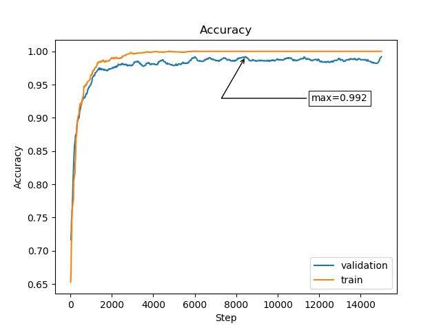
plt.show()After filtering the best result I could obtain was 81.5% accuracy. The next step was to try some data augmentation. Actually, the script we use have some options for augmenting, if you type in your CLI:
$ python retrain.py -hyou find out that there are some options for data augmentation:
- –flip_left_right,
- –random_crop RANDOM_CROP,
- –random_scale RANDOM_SCALE,
- –random_brightness RANDOM_BRIGHTNESS.
But there is a problem with using these options; if you try to turn on even one of them, learning can take 1000 times longer, not just due to the augmentation, but because now the script is not using so called bottlenecks. In short, a bottleneck is an output vector from the “convolutional part” of model, just before last fully connected layer. We can compute bottlenecks for every image and then feed them directly to the last layer of our model. When we use data augmentation, we can’t use bottlenecks because every feeded image is now different. This is big problem, for example, if you want perform a quick experiment locally on your laptop without the GPU, which can increase learning time from 30 minutes to 2 days.
We have developed some compromises to approach this problem. The idea is to generate an augmented dataset before starting learning, and deciding how many times it is to be enlarged. After generating the new datset, we can use bottlenecks again.
In early stages of research, you can test more configurations for augmenting to increase datasets only a couple times, and if you find a solution that meets your expectations you can further increase the number of samples. So whether you have a powerful ML workstation with multiple GPUs, or you use cloud solutions, it still makes sense. This approach allows you to test many more configurations.
Now we have more time to choose another tool for augmenting. Of course for simple augmentations you can use Pillow, numpy etc., but there are some more convenient tools for this task like Keras ImageDataGenerator. I want to show you imgaug. In our case, we need more aggressive data augmentation and imgaug is perfect for this (in the README there is an example showing capabilities of this library). Unfortunately, I can’t find the dataset where such an aggressive preprocessing helps increase accuracy like in ours, so after several attempts I used some basic and common configuration (but I encourage you to test some more sophisticated processing).
import os
from glob import glob
from datetime import datetime
from shutil import copyfile

import imgaug as ia
from imgaug import augmenters as iaa
from scipy.misc import imsave, imread

INPUT = 'flower_split'
OUTPUT = 'flower_augx'
WHITE_LIST_FORMAT = ('png', 'jpg', 'jpeg', 'bmp', 'ppm', 'JPG')
ITERATIONS = 10

def check_dir_or_create(dir):
    if not os.path.exists(dir):
        os.makedirs(dir)

# Sometimes(0.5, ...) applies the given augmenter in 50% of all cases,
# e.g. Sometimes(0.5, GaussianBlur(0.3)) would blur roughly every second image.
sometimes = lambda aug: iaa.Sometimes(0.5, aug)

# Define our sequence of augmentation steps that will be applied to every image
# All augmenters with per_channel=0.5 will sample one value _per image_
# in 50% of all cases. In all other cases they will sample new values
# _per channel_.

augmenters = [
    iaa.Fliplr(0.5), # horizontal flips
    iaa.Crop(percent=(0, 0.1)), # random crops
    # Strengthen or weaken the contrast in each image.
    iaa.ContrastNormalization((0.75, 1.5)),
    # Make some images brighter and some darker.
    # In 20% of all cases, we sample the multiplier once per channel,
    # which can end up changing the color of the images.
    iaa.Multiply((0.8, 1.2), per_channel=0.2),
    # Apply affine transformations to each image.
    # Scale/zoom them, translate/move them, rotate them and shear them.
    iaa.Affine(
        scale={"x": (0.8, 1.2), "y": (0.8, 1.2)},
        translate_percent={"x": (-0.2, 0.2), "y": (-0.2, 0.2)},
        rotate=(-25, 25),
        shear=(-8, 8)
    )
]

seq = iaa.Sequential(augmenters, random_order=True)

files = [y for x in os.walk(INPUT)
         for y in glob(os.path.join(x[0], '*')) if os.path.isfile(y)]
files = [f for f in files if f.endswith(WHITE_LIST_FORMAT)]
classes = [os.path.basename(os.path.dirname(x)) for x in files]
classes_set = set(classes)
for _class in classes_set:
    _dir = os.path.join(OUTPUT, _class)
    check_dir_or_create(_dir)

batches = []
BATCH_SIZE = 50
batches_count = len(files) // BATCH_SIZE + 1
for i in range(batches_count):
    batches.append(files[BATCH_SIZE * i:BATCH_SIZE * (i + 1)])

images = []
for i in range(ITERATIONS):
    print(i, datetime.time(datetime.now()))
    for batch in batches:
        images = []
        for file in batch:
            img = imread(file)
            images.append(img)
        images_aug = seq.augment_images(images)
        for file, image_aug in zip(batch, images_aug):
            root, ext = os.path.splitext(file)
            new_filename = root + '_{}'.format(i) + ext
            new_path = new_filename.replace(INPUT, OUTPUT, 1)

            imsave(new_path, image_aug)

for file in files:
    dst = file.replace(INPUT, OUTPUT)
    copyfile(file, dst)
Example output:
After augmenting, start new training.
$ python retrain.py \

--bottleneck_dir=output/bottlenecks \

--how_many_training_steps 15000 \

--model_dir=inception \

--output_graph=output/retrained_graph.pb \

--output_labels=output/retrained_labels.txt \

--image_dir flower_aug/ \

--learning_rate 0.0001
Accuracy is tremendously better now… actually, it’s a little too good. We made an intentional error to show a problem we might encounter known as Data Leakage.
If you think about one image not as single sample but as some set of features, augmentation mixes up these features. Some are changed, some disappear, some are even created. If we don’t ensure that the validation set is not only variations of images from the training set, a significant part of the features will be present in both sets. In other words — the original image will be too similar to its augmented variants, and these variants too similar to each other.
So we have to split our data into training and validation sets “manually”. The most common way to do this is divide train and validation to separate directories, but we found that it’s problematic to modify this example script to get images from two directories, and it’s easier to write a completely new script. After doing this in Keras, we encountered new problem — we can’t reproduce the accuracy from this example script, with results being 2–3 percentage points lower. We decide to go back to the TensorFlow example script and make as few changes as possible. Instead of using different directories, we added prefix to file names for validation.
First, let’s add a prefix to random images.
import os
import random
from glob import glob
from PIL import Image

INPUT = 'flower_split'
VAL_NUMBER = 4

def get_files(path):
    dirs = [x[0] for x in os.walk(path)][1:]
    files = {}
    for directory in dirs:
        classes = os.path.basename(os.path.normpath(directory))
        files[classes] = glob(os.path.join(directory, '*.jpg'))

    return files

dataset = get_files(INPUT)

for _class in dataset.keys():
    files = dataset[_class]
    random.shuffle(files)
    val_files = files[:VAL_NUMBER]

    for file in val_files:
        basename = os.path.basename(file)
        new_name = 'validation_' + basename
        os.rename(file, file.replace(basename, new_name))
Now we make some small modifications to our augmentation script, so that validation images won’t be processed.
import os
from glob import glob
from datetime import datetime
from shutil import copyfile

import imgaug as ia
from imgaug import augmenters as iaa
from scipy.misc import imsave, imread

INPUT = 'test'
OUTPUT = 'flowers_aug'
WHITE_LIST_FORMAT = ('png', 'jpg', 'jpeg', 'bmp', 'ppm', 'JPG')
ITERATIONS = 10

def check_dir_or_create(dir):
    if not os.path.exists(dir):
        os.makedirs(dir)

# Sometimes(0.5, ...) applies the given augmenter in 50% of all cases,
# e.g. Sometimes(0.5, GaussianBlur(0.3)) would blur roughly every second image.
sometimes = lambda aug: iaa.Sometimes(0.5, aug)

# Define our sequence of augmentation steps that will be applied to every image
# All augmenters with per_channel=0.5 will sample one value _per image_
# in 50% of all cases. In all other cases they will sample new values
# _per channel_.

augmenters = [
    iaa.Fliplr(0.5), # horizontal flips
    iaa.Crop(percent=(0, 0.1)), # random crops
    # Strengthen or weaken the contrast in each image.
    iaa.ContrastNormalization((0.75, 1.5)),
    # Make some images brighter and some darker.
    # In 20% of all cases, we sample the multiplier once per channel,
    # which can end up changing the color of the images.
    iaa.Multiply((0.8, 1.2), per_channel=0.2),
    # Apply affine transformations to each image.
    # Scale/zoom them, translate/move them, rotate them and shear them.
    iaa.Affine(
        scale={"x": (0.8, 1.2), "y": (0.8, 1.2)},
        translate_percent={"x": (-0.2, 0.2), "y": (-0.2, 0.2)},
        rotate=(-25, 25),
        shear=(-8, 8)
    )
]

seq = iaa.Sequential(augmenters, random_order=True)

files = [y for x in os.walk(INPUT)
         for y in glob(os.path.join(x[0], '*')) if os.path.isfile(y)]
files = [f for f in files if f.endswith(WHITE_LIST_FORMAT)]
train_files = [f for f in files if not os.path.basename(f).startswith('validation_')]
classes = [os.path.basename(os.path.dirname(x)) for x in files]
classes_set = set(classes)
for _class in classes_set:
    _dir = os.path.join(OUTPUT, _class)
    check_dir_or_create(_dir)

batches = []
BATCH_SIZE = 50
batches_count = len(train_files) // BATCH_SIZE + 1
for i in range(batches_count):
    batches.append(train_files[BATCH_SIZE * i:BATCH_SIZE * (i + 1)])

images = []
for i in range(ITERATIONS):
    print(i, datetime.time(datetime.now()))
    for batch in batches:
        images = []
        for file in batch:
            img = imread(file)
            images.append(img)
        images_aug = seq.augment_images(images)
        for file, image_aug in zip(batch, images_aug):
            root, ext = os.path.splitext(file)
            new_filename = root + '_{}'.format(i) + ext
            new_path = new_filename.replace(INPUT, OUTPUT, 1)

            imsave(new_path, image_aug)

for file in files:
    dst = file.replace(INPUT, OUTPUT)
    copyfile(file, dst)
Finally we have to modify the training script. I won’t go into much detail, but we added a new argument –prefix_mode and modified the create_image_lists function so that use relevant files to validation. Here is new script.
$ python retrain.py \
--bottleneck_dir=output/bottlenecks \
--how_many_training_steps 15000 \
--model_dir=inception \
--output_graph=output/retrained_graph.pb \
--output_labels=output/retrained_labels.txt \
--image_dir flower_aug/ \
--learning_rate 0.0001 \
--prefix_mode
And results:
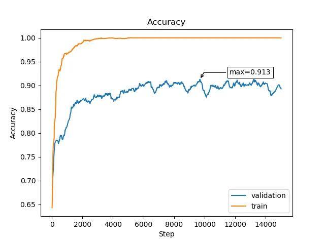
We get 91.3% accuracy, that means that we halved error compared to original dataset.
There are two traps now. First, if you’re doing research and trying some different augmentation configurations, you need to delete old bottlenecks, or switch –bottleneck_dir to other directory. This is because names of the augmented files are the same: input_file_0.jpg, input_file_1.jpg etc. and scripts will find cached bottlenecks for these files, which are made from old files.
The second trap is that, if you are always using the same validation set, you learn how to choose parameters to get the best results for a specific dataset, so you will work similary like machine learning optimizers. Besides changing validation sets, this is a reason you should use also test set.
In general, if your results seems to be too good, there is a good chance that there is something wrong and you have to double-check everything. On the other hand, take a lesson from Millikan’s oil drop experiment and do not overdo the opposite way.
Summary
In this article I wanted to share our experiences and what we learned during our work on machine learning, and summarize some knowledge from different sources. Lack of data is a common problem especially for smaller players, as well as in medical applications due to privacy concerns.
Using the examples, we’ve shown how data augmentation can be useful for small datasets, but we also wanted to draw attention to some pitfalls you might encounter during research and development. We hope that reading this article will help you in your machine learning projects. If you have some observations, different experiences or feedback please leave us a comment or let us know — it will be most appreciated!
References
[1] A. Krizhevsky, I. Sutskever, and G. Hinton. Imagenet classification with deep convolutional neural networks. In Advances in Neural Information Processing Systems 25, pages 1106–1114, 2012.
[2] Christian Szegedy, Wei Liu, Yangqing Jia, Pierre Sermanet, Scott E. Reed, Dragomir Anguelov, Dumitru Erhan, Vincent Vanhoucke, and Andrew Rabinovich. Going deeper with convolutions. CoRR, abs/1409.4842, 2014.
[3] Nitish Srivastava, Geoffrey Hinton, Alex Krizhevsky, Ilya Sutskever, and Ruslan Salakhutdinov. Dropout: A simple way to prevent neural networks from overfitting. Journal of Machine Learning Research, 15:1929–1958, 2014.
[4] Baiyang Wang and Diego Klabjan. Regularization for unsupervised deep neural nets. CoRR, abs/1608.04426, 2016.
[5] Luis P´erez and Jason Min Wang. The effectiveness of data augmentation in image classification using deep learning. 2017.
[6] A. Antoniou, A. Storkey, and H. Edwards. Data Augmentation Generative Adversarial Networks. ArXiv e-prints, November 2017.
[7] H. Inoue. Data Augmentation by Pairing Samples for Images Classification. ArXiv e-prints, January 2018.